
Update: Interested in data virtualization performance? Check out our most recent post, “Physical vs Logical Data Warehouse Performance: The Numbers.”
After my initial post about the topic, I have received several requests to provide more examples of how query optimization works in Data Virtualization, especially in the context of Logical Data Warehouse and Logical Data Lake architectures. Stay with me until the end of this post, and you will understand the most important optimization techniques for these scenarios, namely full aggregation pushdown, partition pruning, partial aggregation pushdown and on-the-fly data movement.
Let’s start by describing the environment we will use for our examples (it is very similar to the one from my previous post). Suppose you work for a big retailer which sells around 10 thousand products. The products data is in a conventional relational database. For each product, the database stores its ‘identifier’, ‘product name’, ‘product category’ and ‘list price’.
The retailer also has a Data Warehouse with sales information. For each sale, the Warehouse stores the identifier of the sold product, the sale date and the sale price. The Data Warehouse stores only sales from the last year, and now it contains approximately 200 Million rows. Sales data from previous years is periodically offloaded to a Hadoop-based repository running Hive (or a similar system), which currently stores around 1 Billion sales. The data fields stored in Hive for each sale are the same as in the Data Warehouse.
In my previous post, we considered the performance of a query to obtain the total sales by product in the last two years. Summarizing what was explained there, the Data Virtualization server can apply the following strategy to answer it:
- It “pushes down” to the Data Warehouse a query to compute the total sales by product in the last year. This query returns one row for each product (10 thousand rows).
- In parallel, it also pushes down to the Hadoop Cluster a query to compute the total sales by product in the year previous to the last one. This also returns one row for each product.
- For each product, the Data Virtualization server adds the partial results computed by each data source in steps 1 and 2, to obtain the total sales by product.
- In parallel, the Data Virtualization server also queries the Products database to obtain the additional data needed for each product (e.g. product name, product category,…) and merges them with the results from step 3.
This is a good example of the full aggregation pushdown technique in action. Although computing the aggregated sum of sales involves processing hundreds of millions of rows, only 30 thousand rows are transferred through the network and processed in the data virtualization layer, and most of the work is performed by the Data Warehouse and the Hadoop cluster, which are systems specially designed for computing large aggregation queries in an very efficient way.
Now, let’s consider some variations of this query:
1. Obtain the total sales by product in the last 9 months
In this case, the query condition allows the Data Virtualization server to know that we only need the sales data from the last 9 months, so accessing Hadoop is not needed and that branch can be entirely removed from the execution plan. This is usually called partition pruning. Combining this technique with ‘full aggregation pushdown’, this query can be resolved by transferring only 20 thousand rows from the data sources to the Data Virtualization server (see Figure 1).
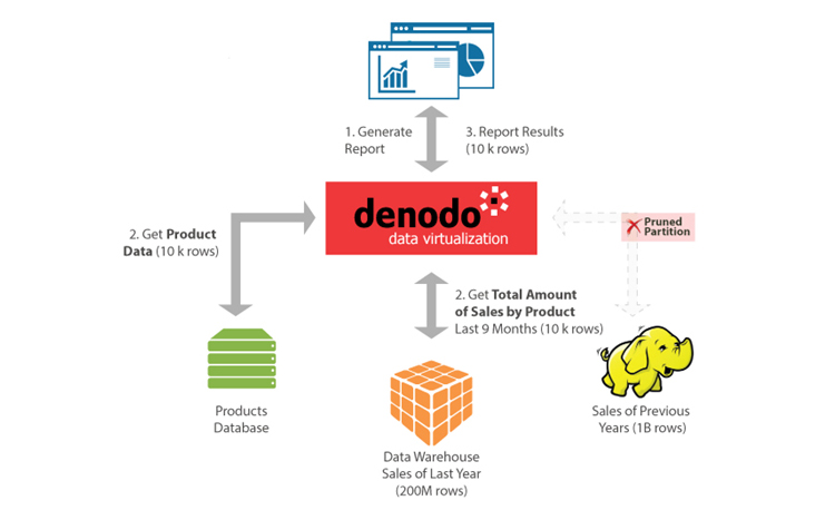
Figure 1: Since the query only involves sales from the last 9 months, the Hadoop branch can be pruned from the execution plan. The computation of the total sales by product is pushed down to the Data Warehouse and the DV server merges the results with the products data.
2. Obtain the total sales by product category in the last 9 months
The main difference with respect to the previous query is that we want the total sales for each product category, instead of for each individual product. As explained in the description of the environment, the information about which category a product belongs to, is stored only in the Products database. Therefore, it is not possible for the Data Warehouse to compute by itself the total sales by category. Nevertheless, the Data Virtualization Server can still apply the following strategy:
- It pushes down to the Data Warehouse a query to compute the total sales by product. This query will again return one row for each product. For instance, if we had 3 products (instead of 10 thousand), this query could return a result set like this:
Product ID |
Total Sales |
| 1 | 1000 |
| 2 | 1500 |
| 3 | 1200 |
This indicates that total sales of products 1, 2 and 3 in the last 9 months are, respectively, 1000, 1500 and 1200 dollars.
- In parallel to 1, it queries the Products database to obtain the correspondences between products and product categories. For instance, if we had 3 products, this query could return:
Product ID |
Product Category |
| 1 | Phone |
| 2 | Phone |
| 3 | Computer |
- Finally, the Data Virtualization Server carries out a join of both tables and sums the totals of all the products in the same category. Following with our example, the this would be the final result:
Product Category |
Total Sales |
| Phone | 2500 |
| Computer | 1200 |
This is an example of partial aggregation pushdown. The difference with ‘full pushdown’ is that the aggregation operation is performed in two steps: one of them is pushed down to the data source (in this example, computing the total sales by product) and the second one is performed by the Data Virtualization server (in this case, obtaining the totals for each category). As this example illustrates, partial pushdown can still be highly effective: this execution plan only requires transferring 20 thousand rows from the data sources to the Data Virtualization server (10 thousand in step 1 and another 10 thousand in step 2).
3. Obtain the maximum discount for each product in the last 9 months
In our final example, we want the maximum sale discount applied to each product in the last 9 months. The discount applied to a sale is obtained by subtracting its ‘sale price’ from the ‘list price’ of the sold product.
Notice that the ‘list price’ is only available in the Products database. Therefore, the discount of a sale can only be calculated after the sales information in the Data Warehouse has been joined with the information in the product database.
For this query, we will consider two alternative optimization techniques: partial aggregation pushdown and on-the-fly data movement. Let’s start with partial aggregation pushdown. In this case, it works as follows:
- Query the Data Warehouse to obtain all the different sale prices for each product. For instance, if we had only 2 products, this query could return a result set like this:
Product ID |
Sale Price |
| 1 | 10 |
| 1 | 9 |
| 2 | 14 |
| 2 | 14 |
This indicates that product 1 has been sold once at 10 dollars and once at 9 dollars, while product 2 has been sold twice at a price of 14 dollars.
- Query the Products database to obtain the ‘list price’ for each product. For instance, if we had two products, this query could return:
Product ID |
List Price |
| 1 | 12 |
| 2 | 14 |
- Now, the Data Virtualization server can compute the maximum discount for each product. Following with our example, the maximum discounts for product 1 can be computed as max (12-10, 12-9) = 3, while the maximum discount for product 2 is max (14-14, 14-14) =0
Product ID |
Max Discount |
| 1 | 3 |
| 2 | 0 |
Let’s now analyze the amount of data transferred with this first strategy. The query in step 1 will return one row for each combination of product and sale price. For instance, if on average each product has been sold at 2 different prices, the query will return 20 thousand rows, but if it has been sold at 20 different prices, it will return 200 thousand. As usual, the query in step 2 returns 10 thousand additional rows.
Let’s go now with the second execution strategy: on the fly data movement. In our example, the Data Virtualization server would apply this technique as follows (see Figure 2):
- It automatically creates one temporary table in the Data Warehouse.
- It retrieves the product data from the Products database and inserts it in the temporary table.
- Now, it executes the complete query (max. discount by product) in the Data Warehouse and obtains the final results.
Let’s now analyze the data transferred with this second alternative. In step 2, the product data needs to be transferred twice: from the Products database to the Data Virtualization server, and from the Data Virtualization Server to the Data Warehouse. Query in step 3 returns one row per product. Therefore, the total number of transferred rows is 30 thousand. In addition, this strategy also needs to pay the cost of inserting 10 thousand rows in the Data Warehouse.
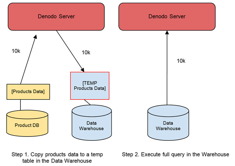
Figure 2: First, Denodo copies the product data to a temporary table in the Data Warehouse. Once this is done, the full query can be pushed down to the Data Warehouse
So, which strategy is better? There is not a fixed answer. It depends on a number of factors such as how many different sale prices we have on average for each product and the cost of insertions in the Data Warehouse. The Data Virtualization server should compare both strategies using cost statistics and determine the best strategy for each case.
Conclusion
As we have shown in this post, even complex distributed queries which need to process billions of rows, can be resolved without moving large amounts of data through the network. Unfortunately, many Data Virtualization systems, especially those from generalist vendors, are lacking (or have very limited support for) the optimization techniques we have described above. Therefore, when building your logical data warehouse or logical data lake project, do not forget to ensure that the Data Virtualization system you choose implements them.
Also interested: Myths in Data Virtualization Performance

- The Rise of Logical Data Management: Why Now Is the Time to Rethink Your Data Strategy - October 22, 2025
- From Ideas to Impact: The GenAI Q&A for Innovation Leaders - June 11, 2025
- GenAI, Without the Hype: What Business Leaders Really Need to Know - June 11, 2025